Leica Lambda Scans

A lambda scan allows you to scan a fluorescent sample across a desired range of wavelengths. This is useful for determining the fluorescent properties of a new dye (and adding it to the dye database) or defining the properties of auto-fluorescence in a sample, so that you can subtract it out of your scans or plan your use of fluors accordingly.

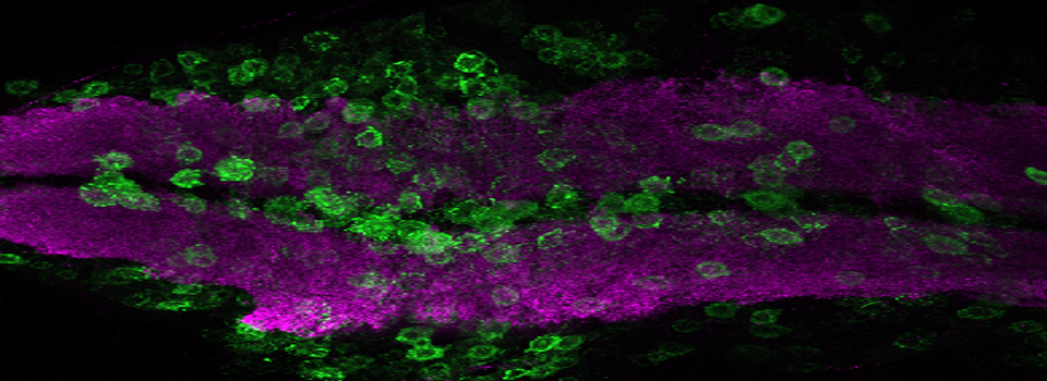
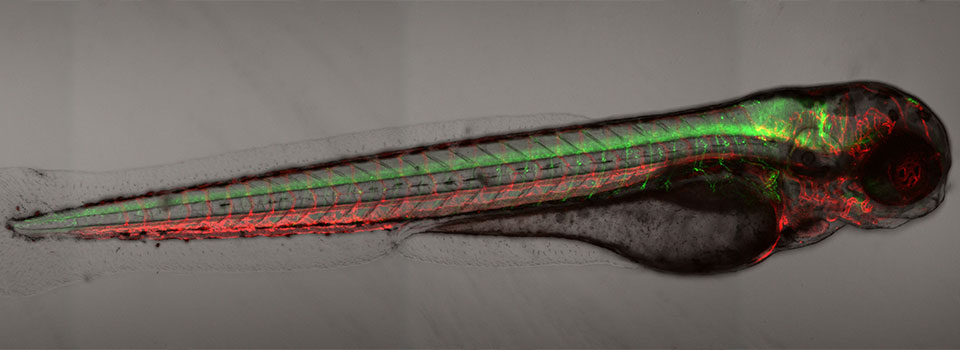
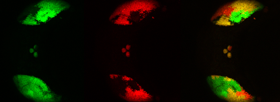
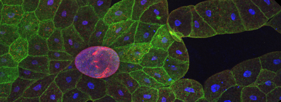
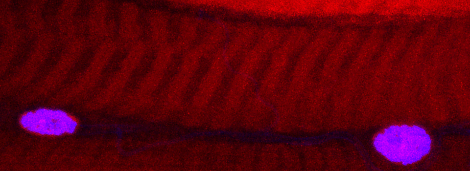
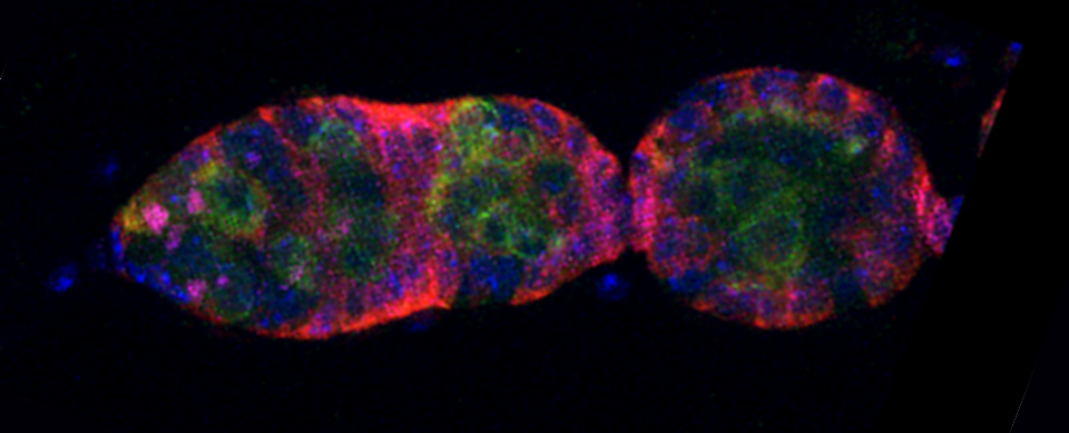
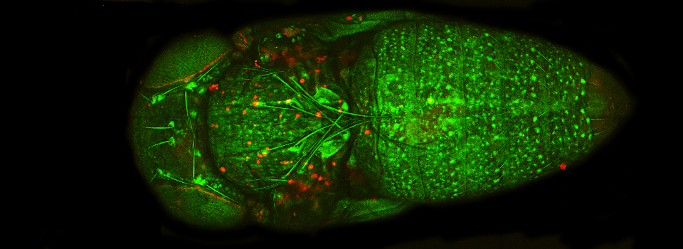
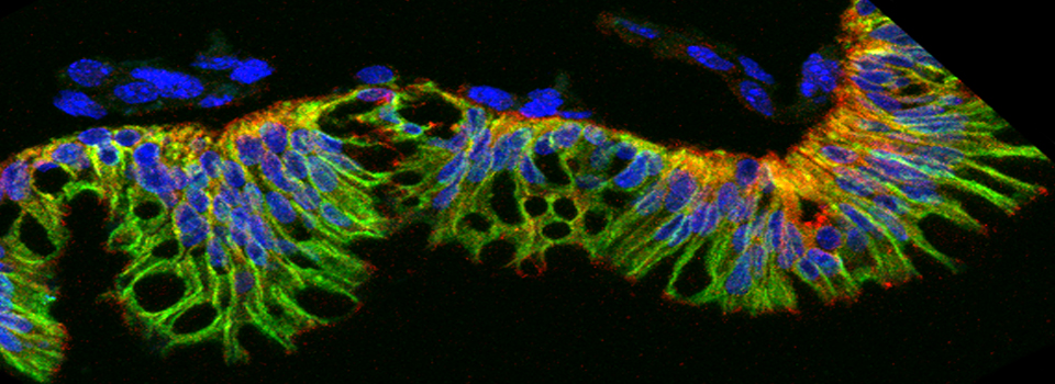
This example shows a scan of a specimen (a Drosophila larva) that has been fixed, embedded in paraffin, and sectioned. This process has caused auto-fluorescence in the tissues.

If you wished to do an experiment that involved staining larva tissues with fluorescent-labeled probes, this auto-fluorescence could interfere. By doing a lambda scan, you can determine the spectral properties of this fluorescence and chose fluors that don’t overlap, or at least have a reference for spectral separation.

Select xyλ from the drop-down menu:

This opens a λ-Scan Range Properties window below:

The spectral display in the center panel will also gain grey bars that represent the detection steps:

“Detection Begin/ End” sets the range of the spectrum covered by the grey bars. The range you use depends on the laser you use. Emission wavelengths are longer than excitation wavelengths, so you need not include wavelengths shorter than your laser line. “Detection Band Width” sets the size of the bars (minimum setting is 5 nm), and “No. of Detection Steps” sets the division of the “Total Detection Range”. In the above example there are gaps between the bars, and this is a reflection of the “λ-Detection Stepsize” being greater than the “Detection Band Width”.

If the scan were to be run with these settings, the portions of the spectra not covered by the grey bars would not be included. To cover those gaps, you can increase the “Detection Band Width” and/or increase the “No. of Detection Steps”.

These settings eliminate the gaps. It is possible to further increase the number of steps or the widths of the bars and have the bars overlap.

Which laser should you choose for your scan? If you are putting a new dye into the dye database, you probably already have information about its excitation/emission spectra. In the case of an auto-fluorescing sample you will have to make an educated guess. A good place to start is to consider the fluorescent labels you are most likely to use in your experiment and test those laser lines first. As an example, consider that you have a choice of either Alexa488 or Alexa633 labeled 2° antibodies to use with the 1° antibody to your protein of interest. Start by activating the argon laser, choose the 488 laser line, find your optimal focal plane, and run your scan.

When your scan is finished, click the “Quantify” tab, then choose “Tools” and the “Stack Profile” option.

You will need to draw an ROI (region of interest) on your image to generate the emission curve. Select sort ROIs in the Tools panel, then Max Projection (yellow arrow) on the display panel. You can use one of the 3 ROI tools (blue line) to draw an ROI; you should pick a region with a strong signal if you can.

Unclick “Max Projection” to generate the graph:

Right clicking on the graph gives you options like exporting the data to the dye database, and generating a picture file or spreadsheet of the graph:

This sample has a very strong emission at ~540nm when excited by the 488 laser. Therefore Alexa488 (which has a peak emission of around 520nm) is not an optimal choice because of the spectral overlap. The next step is to try the lambda scan with the 633 laser:

The graph for the 633 laser shows pretty much no excitation:

Therefore the auto-fluorescence from the sample would not contaminate the fluorescence from Alexa633.

Our Leica SP8 has a choice of 9 different laser lines (405, 458, 476, 488, 496, 514, 561, 594, and 633nm). With this paraffin section, there was strong auto-fluorescence from scanning with the 488, 514, & 561 lasers, moderate to weak emission from 405, 476, & 496 and virtually nothing from 458, 594, & 633. The choice of optimal fluors should be obvious.