At first glance, the Leica acquisition panel looks very complex and scary. There are many sorts of buttons and displays and drop downs to adjust. While there is an initially bewildering array of settings demanding your attention, once you learn what they do, you will have a great about of flexibility and versatility in setting up your imaging experiments. These protocols are provided here as a reference to help you learn these functions in small, more easily digested bits. The acquisition panel entries will break down the panel into its 3 sections and provide an overview of each one’s functions. Operations such as sequential scans, lambda scans or time courses will be covered in more detail in their own protocols.

The left side of the acquisition window allows you choose the type of scan and set the various parameters. The drop down menu at the top left gives you the available scan modes:

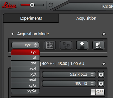
The “x” dimension is the line scanned across the sample by the lasers. “y” is the number of lines scanned. “z” adds the third dimension; it defines the optical plane(s) where x & y are scanned. Modes with “t” allow the user to take a series of images within a specified time span. The “λ” options enable scanning across a range of wavelengths. Choosing an option with “z” and/or “t” and/or “λ” will open specialized panels on the bottom of the left side, which will be introduced below.

The 4 buttons to the right of the scan mode menu are 1-“Define Overview Image” (used to set up a tile scan), 2-“Define Multiple Positions”, 3-“Show Auto-Focus Panel”, and 4-“Show Sequential Scan Panel”.

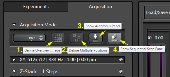
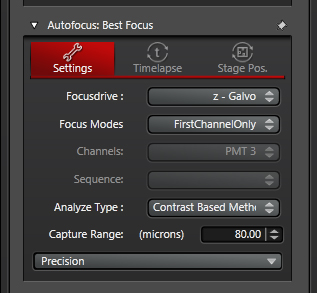
Using functions 1 & 2 requires the scanning stage and will be discussed in another section. The Auto focus panel looks like this:

Here is the Sequential Scan Panel:

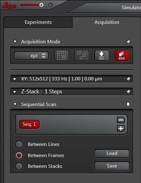
Autofocus and Sequential Scans will also be discussed in more detail in their own separate sections.

The XY portion of the panel is used to set parameters such as scanning speed, frame size, resolution, zoom, etc.:

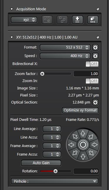
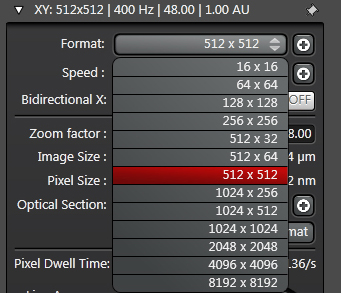
The format menu allows you to choose the size of the xy plane, and the number of pixels you assign to it (your digital resolution). With the 512(x) X 512(y) option you have 512 lines that are subdivided into 512 pixels apiece.

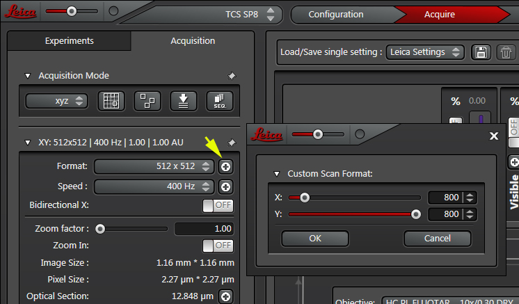
You also have the option to use a custom format. Click the “+” button to the right of the format dropdown to open a new window that allows you to specify the x-y dimensions:

How many pixels should you assign to a line? That will depend on how much resolution you need. A good guideline (from the Nyquist sampling theorem) is that your pixels should be ~2.3 times smaller than the smallest structure you wish to image. Some people might think that more pixels are always better, but there are tradeoffs. Increasing the format means much larger files. There is also the problem of “diluting” the photons; increasing the number of pixels means that you will collect fewer photons per pixel. Of course you can scan at a slower speed or increase the laser power, but that may introduce new complications (photobleaching, damage to live samples). In most cases it’s best to go with just enough pixels to depict what you want to image. The panel will give you a readout of both the pixel size and the image size, as determined by your objective, format, and zoom factor.

The “Speed” menu controls how long the laser(s) will dwell on a pixel.

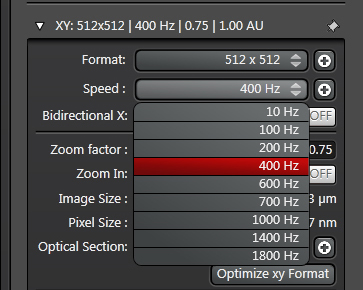
For most xyz scans, a speed of 400 Hz will give you quality images. Slower scan speeds will generate more photons, but also increase the risk of photobleaching fluors and damaging live samples. The faster speeds are most often used for live imaging (see the section on time scans). As with the format, you can click the “+” button at the right to choose a custom scan speed (up to 1800 Hz). The middle of the XY panel will give you the pixel dwell time and the frame rate (how long it takes a laser to scan all the pixels in the field).

The “Bidirectional X” option allows the laser to scan the x dimension both in the forward and the return motion. This option is useful for live scans when you are recording fast events as this will double your speed.

The zoom factor setting allows you to zoom out (to 0.75x) or zoom in (to 48x).

“Zoom in” allows you to draw a square ROI anywhere on your field of view, and enlarge that region.

Line averaging can be very useful for enhancing a weak signal. The laser will scan a line, then scan it again and average the photons counted per pixel. The next repeat scan will be added to that average, and the total re-averaged, for as many repeat scans as are specified:

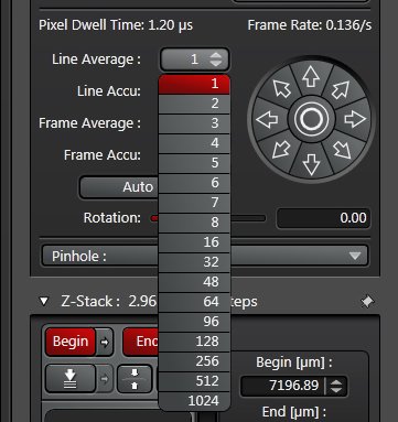
You probably won’t ever need to set this higher than 4 or 5.

Line averaging helps boost your signal relative to the noise, but it will increase your scan times and can up the risk of photobleaching.

Line Accu will add all the scans of a line together. That also makes a signal stronger, but it will boost background signal too. Frame Average and Frame Accu will average or add together individual scan cycles (repeat scans of xy optical sections).

The circle with the 8 arrow buttons will allow you to move the scan field in the direction of the arrow clicked. This function can only be used if you have a zoom factor selected that is larger than then minimum permitted. The round button in the center moves the view back to where it started. The Rotation slider allows you to rotate the angle of the scan field. It does not move the specimen.

Most users will never need to deal with the pinhole setting:

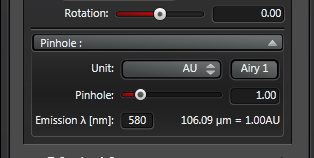
The pinhole allows the system to collect the in-focus light from the chosen optical plane and exclude the out-of-focus light from the other planes. The default setting is 1 Airy Unit (AU), which is optimal for the vast majority of applications. If you shrink the pinhole, you can gain a modest increase in resolution, but at the expense of collecting less light. On the flip side, a larger pinhole settings allows more light to pass, but deceases the resolving power of the system.

Here is a quick glance at some of the dimension-specific panels (covered in greater detail in their own sections).

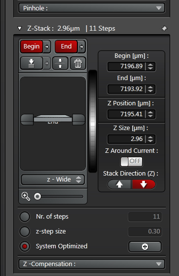
Scan modes that include the z dimension will open the Z-stack panel:

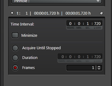
Here is the panel used for setting time parameters:

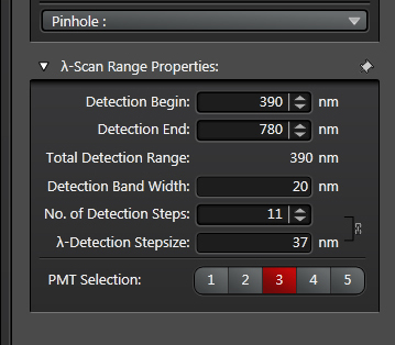
And finally, the lambda scan panel: