The Sensitized Emission (SE) method of FRET measurement uses measurements of controls in addition to the FRET pair to compensate for issues such as spectral crosstalk, differences in fluorescent protein expression, and background noise. In contrast to the acceptor photobleaching method, it is much less invasive, and therefore a better choice for live imaging. It can also be used with fixed specimens.

To run the necessary calculations with the FV1000 FRET SE module, the following images are needed:

You will need 3 specimens to image: one with the FRET pair, a Donor only control, and an Acceptor only control.

Collecting the data

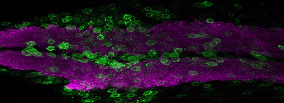
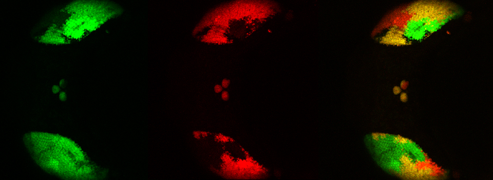
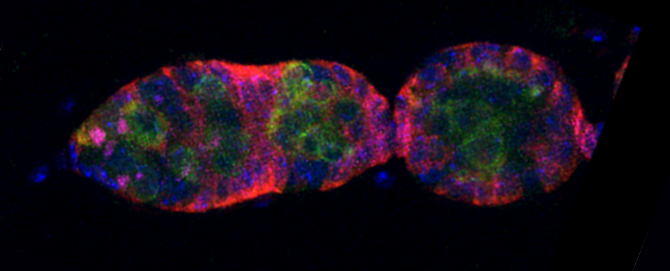
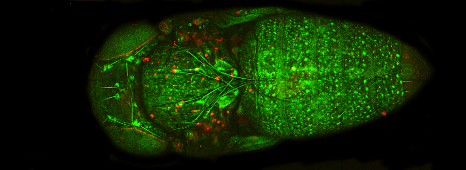
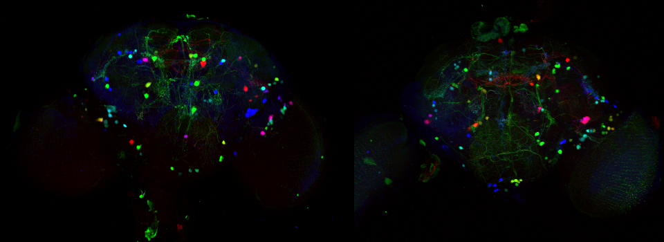
In this example, I am again using the CFP-EPAC-YFP FRET sensor, expressed in adult Drosophila brains with the OK107-GAL4 driver. For the 2 controls I have used brains from OK107-GAL4 > UAS-EYFP or OK107-GAL4 > UAS-ECFP flies. These specimens have been fixed.

The data is collected in standard confocal scanning mode, and the FRET SE module opened afterwards for data analysis. Load “ECFP_458” and “EYFP” into the dye selector to set up a channel for each fluor. You should keep both channels active for all the scans, and switch between the 458 nm and 515 nm lasers as required. The images collected for this demonstration to be loaded into the SE calculator were:

a* OK107>ECFP 448 nm laser ch1 b* OK107>ECFP 448 nm laser ch2 c OK107>EYFP 448 nm laser ch2 d OK107>EYFP 515 nm laser ch2 e+ OK107>EPac 448 nm laser ch1 f+ OK107>EPac 448 nm laser ch2 g OK107>EPac 515 nm laser ch2

(*, +- note that a & b, and e & f can each be collected with the same scan)

Here is the set up for the scan that collected images “e” and “f” from the FRET slide (OK107> EPac):

For this scan the 458 nm laser (cyan *) is activated, and the 515 nm laser (yellow *) is turned down to 0%. Channel 1 shows the CFP signal (“e”) from direct excitation from the 548 nm laser, and Channel 2 the YFP signal from FRET and some uncorrected crosstalk (“f”). The name of the .oib file includes “e, f” to make loading into the FRET SE module easier.

The next example shows the changed settings with the same specimen to collect image “g”:

This time the 458 nm is dialed to 0% and the 515 nm is activated. The HV is channel 2 was lowered from 460 to 345 to avoid oversaturation of the image. The CFP image (channel 1) will not be used for FRET calculations, but it provides a record that the CFP was not excited above background by the 515 nm laser.

Repeat the scans with the Donor only and Acceptor only controls (a-d), using the laser lines listed above.

Analyzing the data

Once you have collected all the required images, you can open the FRET SE module,

which opens this window:

In order to load the images, the data files must be opened with the FV1000 software.

Each place for uploading of images is marked with the letter code, starting with “e”.

If you check the button next to “Use the same image as donor” for panel “f”, you can load both “e” and “f” together. Make sure Ch1 is selected for “e” and Channel 2 for “f”.

After images e, f, and g are selected, the next stage is doing background subtraction for each one. This example will use the “Value” option.

To determine the background threshold, open the image and draw a small square ROI in a region without your signal, in this case a portion of the brain outside the mushroom body regions where there is some background signal. Then click the “Measurement” button.

Plug the average value for ch1 into the background panel for image “e”, and use the value for ch2 for image “f”. Repeat this process for image “g”.

Now set the Forster Distance value for CFP-YFP:

Next click the “Calculation parameter” button:

Check that the correct quantum yield values are set for CFP (Qd = 0.87%) and YFP (Qd + 0.57%). The Output range will affect the look of the color map the SE FRET panel will generate. The example here will show a FRET efficiency range from 0-100, and a show distances between flours that range from 0-10 Angstroms.

Finally, load images for the 4 single fluor controls. Make sure you select the correct channel (*) for each:

Clicking the “Execute” button will generate a new .oib file with the FRET heat map data: