Most people using the confocal microscopes will be taking simple Z-stacks (XYZ scan). This section will cover those, and how to do basic time-lapse (XYT or XYZT) imaging. The focus here will be on the most commonly used windows and adjusted settings.

The LSM Imaging window:

1) Scanner type controls. Most scans will use the standard Galvano scanner. If you intend to do time-lapse scans of something moving fast, or you wish to reduce laser exposure on a delicate specimen, you can opt for the Resonant Scanner.

2) Scan speed. 2 microseconds per pixel is the default setting and works fine for most imaging. You can opt to slow the laser down by adjusting the speed with the slider. This will boost your signal but also increases the risk of photobleaching. The Resonant scanner goes 30 fps at 512x512 pixels and 438 fps at 512x32 pixels).

3) Aspect Ratio. This controls the shape of your field of view (FoV), square (1:1) or rectangular (4:3).

4) Scan Size. This controls your digital resolution. 512 x 512 (512 lines divided into 512 pixels each) is the default setting. Depending on your imaging needs, you may wish to increase or decrease the number of pixels. The pull down will give you those options.

The Area Settings Window:

1) Zoom. This allows digital magnification of your image. You can control it by clicking the arrows (fine control) and clicking and dragging the bar (coarse control).

2) Optimize. This calculates an optimal zoom setting based on Nyquist calculations. The small red arrow on the zoom bar indicates the value. The Nyquist value location will vary depending on the objective used and the number of pixels selected with the Scan Size setting. You can zoom past this point, but you will not gain any improvement in resolution.

3) X1. This resets the Zoom value back to 1x.

4) Rotation. This allows you to digitally rotate the FoV by left clicking and holding on to the blue dot, then rotating the circle (representing the FoV seen through the objective) to the left or right. The square within the circle is the digital FoV. This is useful for specimens like embryos that have distinct axes and need to be aligned.

5) Pan X/PanY. These controls can be used to make fine X-Y adjustments to the location of a zoomed FoV within the original FoV.

6) Reset. Undoes Rotation/PanX/PanY changes.

The PMT Setting Window:

1) Mode. Most experiments will be in the “VBF” setting.

2) Averaging. This feature improves signal to noise by repeating a scan of a line (or a whole XY frame) and averaging the pixel intensities. This does add to the total scan time but usually improves image quality. 2-3 repeats are usually sufficient.

3) Sequential Scan. If “None” is selected, all active lasers will scan simultaneously. Most scans are done with this feature activated, because of overlapping emission spectra of commonly used fluors (the overlap between DAPI and GFP/FITC/ Alexa-488 being a common problem). You should select the “Line” option if your scan has a time dimension; otherwise choose “Frame”.

4) Dye & Detector Select. This button opens a new window for setting up the detectors. More on this below.

5) Confocal Aperture. This controls the size of the pinhole, which is set to 1 Airy Disk as a default. You can increase the pinhole opening to collect more light or reduce it to gain a bit of increased resolution. Reducing more than 50% hits the law of diminishing returns.

The Dye and Detector Select Window:

This window is used to tell the software which dyes are to be detected and set the detector parameters. The list of dyes is on the left, with a short list of recently used dyes above, and the complete list below. Click to highlight a dye (in this example Alexa Fluor 488), then click “Add”. If you cannot find your exact dye on the list, pick one with a similar spectrum.

Repeat this with each dye you want to add.

TD is the channel for transmitted light (DIC brightfield). It will be assigned to the group with the highest wavelength laser. If you don’t need a brightfield channel, highlight it and click “Remove”. Click “OK” to finalize the dye selection.

If you have “Sequential Scan” active, all the dyes will be assigned into separate groups (1). Only one group can be scanned at a times, but you can toggle freely between groups during a live scan.

1) Group layout. This shows which detector each channel is assigned to and allows you to select a group to image in live scan mode.

2) Laser Filter. This gives you the option to set a 10% ceiling on laser power. Most scans work fine under this threshold.

3) Laser power control (for Channel1/group 1 in this example). You can click and drag the bar for coarse control of the laser power. Use the arrows for fine control.

4) HV. This is the amount of voltage to the detectors. Increasing it increases signal strength but going above 750 risks adding noise to the image.

5) Gain. This will multiply the intensity of a signal, but it will also increase background too.

6) Offset. This “raises the floor” of the dynamic range by resetting the value of the zero pixel. 3 the recommended default setting. You may find that a higher or lower offset is optimal for your image.

7) Detector range. This shows the wavelength range of emitted light that is measured by the detector (430-470 nm in this example). You can adjust this by typing in new numbers or moving the corresponding color bar in the Spectral Setting window (red arrow). You are limited to a maximum of a 100 nm range, and you should take care to keep the lower limit at least 6 nm larger than the laser line.

Once the detectors are assigned, you can start live scanning your specimen. This is just like looking through the eyepieces; you can see an image and make adjustments, but you are not recording data.

The Imaging Window

This is the largest window in the center of the screening. If there are no images open, the controls on the top left look like this:

1) Live Tab. This is always at the top left of the window. This is the tab that needs to be active for live scanning.

2) Live Scan controls. “Live” will scan each line. “Livex2” scans every other line, which allows for faster scanning at a slight reduction in live image quality. You should not use this or “Livex4” if your dyes are very sensitive to photobleaching. “Livex4” scans every 4th line.

3) “Hi-Lo”. This shows the range of pixel intensities on the image.

Locate, position, and focus on your specimen via the eyepieces before you live scan via the computer controls. Here is an example of a live scan of Channel 1:

Adjust Laser Power and HV for channel 1 until you see an image. You may also need to adjust the fine focus knob, as your eyes looking through the eye pieces may not have the same focal plane as the scanner. Here is the image in Hi-Lo mode:

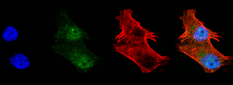
Blue represents a zero-value pixel. Increasing intensity is represented through gradations of black through many shades of grey thought white to red (saturated pixel, 4095). You should avoid large patches of red pixels on your image; this is oversaturation and obscures detail. Over-exposed images cannot be corrected via post-imaging processing, so this is where you should take the time to properly adjust your settings.

Repeat this process with the rest of your channels.

If you are using DIC, it will share a laser with a fluorescent channel, and adjusting the laser will affect both. There is another tab for bright field adjustment: the Ocular Window. There are 3 things you can experiment with to see if you can enhance contrast.

1) Polarizer. This filter will exclude light, so you will need to increase the detector HV setting after turning it on.

2) DC Prism

3) DC Prism Contrast slider

You will need to experiment with turning these settings on/off to see which works best for your specimen. Here is the effect of activating the polarizer:

After increasing the HV:

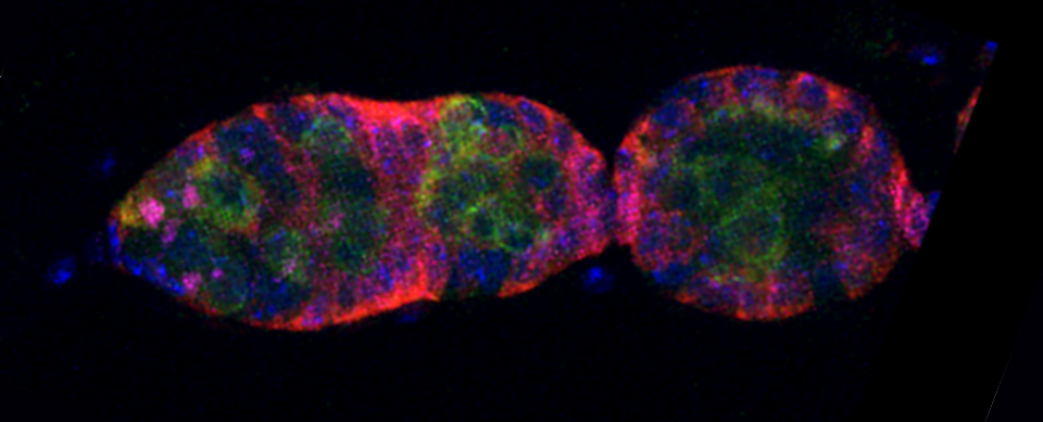
Activating the DIC prism improves the contrast of this specimen even more, particularly in the nurse cell nuclei:

Once you have adjusted all the channels to get a signal, you can set your Z-stack range. You will need to choose a channel, and usually the best option is a channel that covers the most depth in a specimen. For example, if you are imaging cells, it is better to choose a cytoplasmic stain over a nuclear stain, since there will be cytoplasm over and under a nucleus. Likewise, a membrane stain will cover more depth than a cytoplasm stain. For some specimens, such as this fly ovary, there may not be a great difference in distance spanned in the Z-axis between the channels.

All channels will have the same range in the Z dimension once it is set.

This is the Series Tab:

To enable the Z dimension, click the ON button (1). (2) shows the current Z coordinate. Once you can a focus on your specimen, you have the option to Register its location on the Z axis (3). This is a place marker for your focal plane. If you turn a focus knob too far and lose your place, you can click the “Move” button (4) to return to that focal plane. The Optimize button will set the Step size ( (9)-thickness of your optical slice) based on the resolving power of the objective. You should click this if you change objectives, as the software will not automatically change it for you. (6) and (7) set the start and end coordinates of a Z-stack. Once you set your stack, the window will show you the number of slices (8), which is determined by the Step Size (9) and the range of the Z-stack. You can change these numbers by highlighting them with the mouse and typing in a new number: for example, you might not want the 1052 slice Z-stack shown, so you can directly lower it or increase the step size. For some experiments (using the Co-localization or Deconvolution functions in CellSens) you usually want to oversample in Z (2.3x for Nyquist sampling) so you can increase the number of slices or decrease the step size.

To set your Z range, turn the focus knob while live scanning until the signal disappears (only blue and black pixels in Hi-Lo mode). Register the starting point. I prefer to raise the objective and start my stack at the top but doing it the opposite way works just as well. Being consistent in how you set the Z-stacks will result in quicker and more efficient imaging sessions. Turn the focus knob to lower the objective; the specimen will come back into view and fade again as you move past the specimen focal planes. Register the end point.

You should check the Z-range in the other channels to ensure that there are no oversaturated (red in Hi-Lo mode) regions. Use the “Move” buttons to go to the start or the end coordinate of your Z-stack.

The software will calculate an estimated scanning time (*). It is influenced by setting such as number of channels, sequential scan mode setting, number of Z slices, laser scan speed, and amount of line averaging. Click “LSM Start” to records your image.

When the recording starts, a new tab (red arrow) will appear to the right of the other tabs in the image window. The Acquire tab will show Z-slices completed (1), and time remaining in the scan (2). If you need to abort the scan, click “LSM Stop” (3).

The system is saving the data file (to the designated destination) as it scans.

Once the scan is complete, click the tab for the new image file (1). Use the “Z Intensity Projection” button (3) the merge the Z-stacks:

There are several options for viewing the image. “Tile” is the default setting, which shows each individual channel and a merge of all channels. “Single”, “ThreeSides”, and “Volume will give you one large, merged image, and the option to turn each channel on (visible) or off (hidden). In this example the brightfield channel (CH5 TD) is off.

ThreeSides (1) allows you to do virtual sections through your data stack. It works best with large Z-stacks, and oversampling in Z often helps. Usually you will want brightfield off (red arrow), as this shows fluorescent channels best. The yellows lines (2) denote the locations on the main X-Y-Z image of the virtual X-Z and Y-Z sections, shown at the bottom or to the right. These lines can be moved around by clicking/dragging with the mouse. If you are planning to use this view function, it is a good idea to use the Rotate function before imaging to line up the regions of interest with the X-Y axis, as you cannot do virtual sections at different angles.

“Volume” displays a 3-D rendering of your image. It also It works best with large Z-stacks and the TD channel off. The 3-D effect is best seen when the image is rotating slowly. You can start this by grabbling unto the frame around the image with the mouse and “spinning” it (which becomes obvious with a little practice). To make a video recording you will need to open the “Viewer” portion of thew software (red arrow). More detailed instructions to be posted in the future on a separate page.

(Up next: Virtual Phases)