How to do Mosaic Stitching with the Olympus FV1000
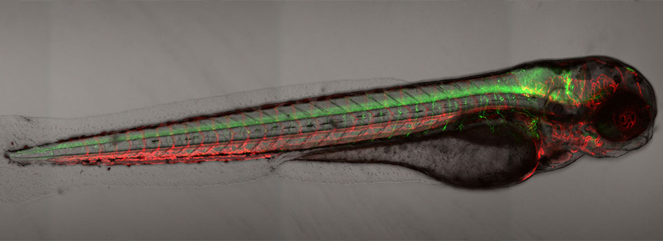
Many samples are larger than the microscope’s field of view, but sometimes you wish to produce an image that shows the whole sample. Mosaic stitching allows you to take a series of overlapping images and merge them together into a seamless picture of the entire subject.
Set up MATL mode
BEFORE you place your slide/dish on the microscope, start the FV1000 software, and select “Multi Area Time Lapse” (MATL) from the “Device” tab on the top of the screen.

The “XY stage warning” window will pop up with the statement: “This stage will move in a wide range to detect its mechanical origin”. Click “OK”. This will cause the stage to move around. When it is finished moving, you can place your slide/dish on the stage.
You should see 3 new windows: Stage Control, MATL Control, and Registered Point List (more detail on those later).
Set up your scan parameters
Load your dyes (virtual phases cannot be done in combination with MATL), find a region of interest on your slide, set exposure levels, etc. If you wish to merge Z-stacks, set your start and end points, then click the “Depth” button in the “Image Acquisition Control “ window. It is essential to click “Depth” BEFORE setting up your matrix, otherwise the program will function only in 2 dimensions.
If you experience a problem with getting the MATL program to accept Z-coordinates, follow the instructions HERE..
If you want to do Time Lapse, see below (“Setting up time-lapse mosaics”).
Set Destination for saved files
Click the 4th button from the right (disc & wrench) on the Registered Point List window, which will allow you to set the folder destination (Folder Name window). You also have the option to name your image files (this will show up later on the Registered Point List spreadsheet).

Set overlap
The 3rd button from the right on the MATL Control window opens the “Preferences” window. Click the “Index Size” tab. The overlap setting is in the window next to the % sign. 100% = 0 overlap. Some overlap is required for optimal image stitching to produce the most seamless combined image. The optimal amount of overlap is determined by the total magnification:
((Obj. mag. X zoom#)/ 8 ) + 3 = ideal overlap%
For example, if you are using a 60X objective with a zoom of 1.5, the ideal overlap is around 14%, and you would set the overlap # to 86%.

If you must do any quantitation on your images, you cannot use overlap. You can still do stitching, but seams are possible in the final image.
Set scan order and pattern
Click the “CoordCreateDir” tab:

The “Normal” scan pattern is recommended.
Define your matrix
The MATL Controller window displays a grid. Each square on the grid represents the x-y plane that can be imaged through the objective. The yellow crosshair shows the position of the sample in the view field on the grid (“you are here”). The red cross marks the center of the grid. The x y coordinates of the yellow crosshair (relative to the center) are shown to the right of the grid (and in the windows of the stage controller). You can zoom in or out with the slider bar to the right. The stage controller allows you to fine control x-y movement from the computer. The windows at the top are particularly useful as they will allow you to go back to any set of coordinates on your side. When you find a region of interest, it is a good idea to jot down the coordinates in case you stray too far from it. You can also double click any square on the MATL controller grid to move the field of view to that position.

You have 2 options for setting a matrix. The “Define Matrix” button (3rd from the left in the MATL Controller window) will allow you to specify a set number of squares across and down.

Click “Set” and the yellow crosshairs will be centered in the defined matrix. The coordinates for each square will be loaded into the Registered Point List.

The “Mosaic Outline” button (2nd button from the left on the MATL Controller window) will allow you more direct control over the location of the matrix, but all the points must be entered manually. If you define an irregular matrix, the program will fill in squares to create a rectangle. Click a square you want included, and then click the “Mosaic Outline” button. A window (“Mosaic Outline”) will open that will show the coordinates of each entered square. Click the 1st button (red on black) to enter the coordinates. Click on the next square on interest in the MATL Controller window and repeat. When you have entered all the squares, click “Apply” in the “Mosaic Outline” window. The coordinates for each square should then appear in the Registered Point List window.

Take images
You will use the start controls in the “Registered Point List” window instead of the “Image Acquisition Control” window. First click the “Ready” button (bottom left). When the machine is ready to start, the next button, “Play”, will change from a grey arrow to a black arrow. Hit “Play”. You should see windows appear for all your channels in the “Live View” window. If you are Z-stacking you should see a z-stack # indicator below the “Ready” and “Play” buttons in the bottom left corner of the Registered Point List window. “Total Time” (bottom right) gives you an estimate of how long the scan will take. The system will scan the entire Z-stack for square 1 (if applicable), then move to the next square.

Finding the right stitch
When your scan is finished, go to the “Device” tab and select “MATL Viewer”. This opens a new window with a picture of imaged squares. Click the 4th button (“Select view mode”) and select the bottom button (green tiles) on the drop down menu.

This should arrange all the images in their proper order.

To generate a stitched image go to the 3rd button on the MATL Viewer (“select action) and pick the 6th button (“stitch”) in the drop down menu.

This will open the “Stitch View” window. Click the “Show” button to generate an initial stitched image in the window. Finding the ideal stitch requires a bit of trial and error. If you are stitching Z-stacks, using a plane in the center will usually give you the best results. Use the Z slider to the left to pick a Z plane, and then hit the “Show” button to re-stitch. The channels used are indicated above the stitched image and will be initially all checked. If the image is not optimal you can uncheck some of the channels and re-stitch. The channel with the most contrast works best for guiding stitching. Try different Z-planes and channel combinations to find the best possible image. You can also try stitching with and without the “Correction” and “Smoothing” options checked to see which stitch trial is most to your liking.

Saving the data
Once you generate a stitch you wish to keep, click the “Save As” button on the bottom right of the Stitch View window.

If you are saving a Z-stack stitch, you must check “Apply to series” to add all of your stacks to the image. Files 1 GB or less can be saved in the “oib” format. Files larger than 1 GB should be saved as an “oif”. If you have Z-stacks and/or 20+ tiles you will likely choose “oif”.
Your saved data will look like this in the window:

Clicking on an “oif” opens a 2D View window.

If you wish to go back and re-stitch from the raw data, open one of the “FV10_” (or whatever you have named them) folders through the MATL viewer window:

Click on the “MATL_Mosaic” file to open a new “Stitch View” window.
MATL with well plates
The Olympus software also allows a user to program an automated scan of well plates. You can set the system to record mosaics in the specified wells.
1) Put on the well plate stage insert, select “Multi Area Time Lapse” (MATL) from the “Device” tab on the top of the screen, and initialize the stage. Do NOT put on the well plate until AFTER the stage has finished moving.
2) Focus on a sample in one of the wells, and set your scan parameters as mentioned above.
3) Next you will specify the type of plate you are using. You can pull up the “Well Plate Setting” window from the options menu on the MATL Controller window, or click the “Set Well Number” icon:
![]()

Glass bottomed plates are required for the best quality images (i.e., to use the oil objectives. You can use plastic plates with the air dry objectives.). The Olympus software already has the settings for Greiner plates. If you use a different brand of plate, you will need to fill in the dimensions (column and row numbers, height, width, and pitch). Select “User Custom” from the “Well Name” drop down menu.

Click “Apply” and the well positions will be added to the stage map (the example shows a 96-well plate):

You can erase the purple circles by choosing “None” in the Well Name menu. If you program in custom settings, the software will remember that last set entered.
4) When you set your file destination, click on the box for “Add Well position before folder and file name”. This will make sorting through your data files, much, much easier.

The rules for assigning a scan to a well:

5) Your last step in specifying your plate is to register the centers of the wells. Click on the red cross on the Stage Controller to move to the center of the plate. You can select “Register Well Position” from the Edit menu on the MATL Controller window, or click the “Register Well Position” icon:
![]()

Click “Next”, which will change the window to:

Make sure “Auto Escape” is checked, then click “Go to A1”.

The field of view is now in the center of well A1. Click “Register”.
6) You are now ready to set up your matrices. You can opt to scan a matrix in every well, or just in selected wells. Pull up “Define Matrix” from the Edit menu on the MATL Controller window, or click the “Define Matrix” icon:
![]()

When you check the “Register in Multiple Well Plate” box, you will get a new window:

You can select the whole field, rows, columns, or click on individual wells. Activated wells will turn green:

Click “OK”, and then “Set” on the “Define Matrix” box. This will register the matrix coordinates on the stage map and Registered Point List window:

7) Hit the ready button at the bottom left of the Registered Point List window and click the black “play” arrow to start your scan. When you access the MATL Viewer, there will be a dropdown menu (MosaicNo.) at the upper right for each well scanned:

The mosaics will be numbered according to the order selected for scanning the wells. In this example 1 = A1, 2 = A2, and 3 = B1. You will have to play with each mosaic separately for stitching and saving as OIB/OIF files.
Setting multiple matrices within a well (or multiple wells)
If you want to program multiple, unconnected matrices within a well, you can specify them as groups. Position your specimen, set levels, the Z-limits, etc., then open the “mosaic outline” window (1), and set the first x,y coordinate of your matrix (2).

Go to the other side of the specimen and set the next x-y coordinate (1). Click the “add group” button (2), and “yes” in the pop-up window (3).

The software will fill in the matrix between the 2 points you set. In this example, the group is a 1 x 3 matrix:

Go to the next specimen with the stage controller and repeat this process. Once you have added the second group, you can see that end group is represented in the multi area time lapse controller window with a dot for each x,y tile (red *), and a green line that denotes the movement of the stage between matrices:

You can add as many groups as you need, even in other wells:

Setting up time-lapse mosaics.
If you want to do xyt or xyzt scans of mosaic tiles, you should NOT use the “time” button in the “Image Acquisition Control” window. Instead you will control the time setting in the bottom of the “Registered Point List” window:

Time is the last thing you will specify in your mosaic tile programming. Type in the number of repeats you want (red arrow). Once you do that, the interval window to the left will change to reflect your “speed limit”, i.e., the minimum interval between repeats (cyan *). This limit is determined by a number of your previous setting, including your scan speed, digital format, number of Z-slices, number of channels, and size/ number of matrices. You can type in larger intervals in you wish to repeat your scan patterns less often. If you need to go faster, you will have to tweak the other settings to make each scan take less time. Once you have all your desired settings, click the “ready” button. The software will calculate the time needed to do the entire time course, and the start button (cyan arrow) will change from grey to black.
The picture below shows what the “Registered Point List” window looks like during an xyzt scan of the 3 groups of 1 x 3 matrices set up in the example above. The matrix coordinate currently being scanned will be highlighted in blue (in this case the 2nd square of group 1). The current Z position is on the bottom left corner (slice # 5 of a stack of 7), and the time panel indicates that this is the 1st scan of 13 time points, with an interval of 2 minutes, 13.2 seconds between scans. A scan pattern is a scan of the full Z-stack for point 1, move to point 2 and scan that full Z-stack, etc. all the way to the last point.

When you activate the Multi Area Time Lapse Viewer, each group will have its own number in the “Mosaic No.” dropdown (red arrow), and each time point can be viewed with the slider (cyan arrow).

In the stitch panel, the times points are indicted/ controlled with the “Repeat” slider (cyan arrow), rather than the “T” slider:

Finally, when saving an XYZT mosaic as an oib/oif file, you must click both “apply to series” and “apply to repeat” to get the complete Z and T stacks. The “set repeat range” section at bottom of the panel allows for cropping in the T dimension, if desired.

MATL without stitching
If you wish to image 3 or 4 dimensional data stacks that are not contiguous and will not be stitched together, use the “Add Current Position” button, which can be found on the top left of the MATL Controller window or the Registered Point List window.

Click this button to add each new imaging location once you have decided all your scan parameters (x-y coordinates, Z stack range, HV and offset levels, etc.). The map of your scan will look something like this, with single dots to denote the x-y coordinates:

Once your scan is complete you will use the MATL Viewer to access your files.

But instead of the “Stitch” button, use the “Open 2D Append Image” button.

This will open an ”Append Range Selection” window:

You can crop time points here if you wish. Clicking OK will open your 3D or 4D data set in the 2D viewer.