The FRET sensitized emission method is suitable for measuring FRET in both live and fixed specimens. Unlike acceptor photobleaching, it is non-invasive, so this is a preferred method for live imaging. Individual controls for both the donor and the acceptor fluors are required to correct for excitation and emission crosstalk. To properly calibrate the system to measure FRET, it is necessary to first preform reference scans of donor and acceptor together, donor in the absence of acceptor, and acceptor in the absence of donor. It is critical that scanning parameters such as gain, emission detection window, excitation intensities, zoom, format, scanning speed, and pinhole diameter are the same for all scans in an experimental run.

Select FRET SE from the down-drop menu:

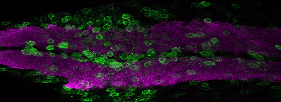
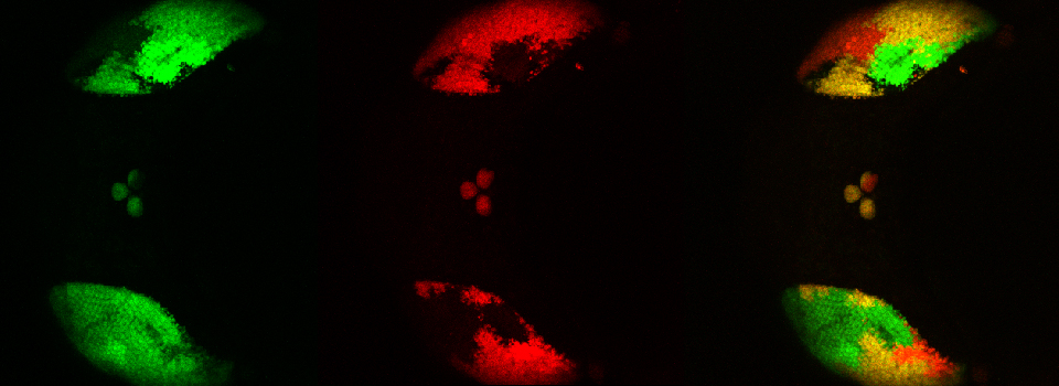
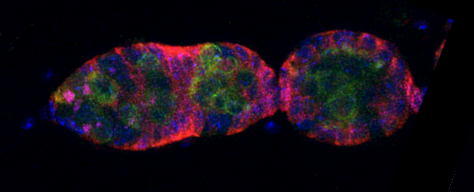
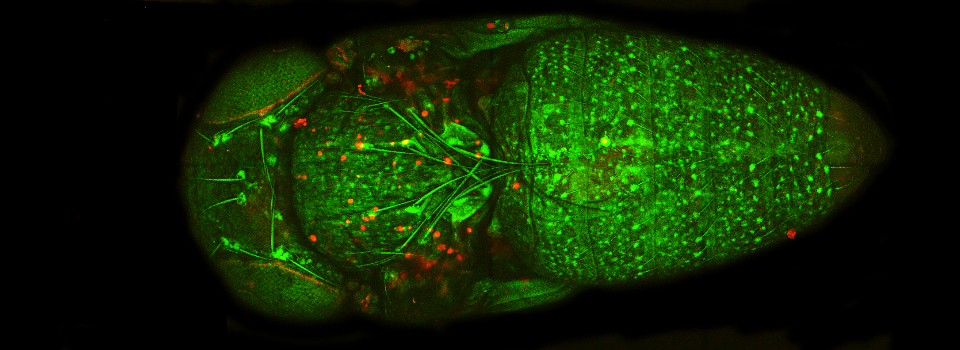
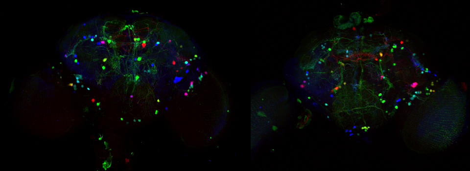
Your first specimen should be a positive FRET control. In this first example, I am using a fixed adult Drosophila brain with the CFP-YFP EPac FRET sensor in the mushroom bodies. Activate the “Donor + FRET” button (Yellow *) and the 458 nm and 514 nm lasers (yellow arrows). Set the detection ranges for CFP (462 nm- 504 nm) in PMT 1, and YFP (524 nm- 580 nm) in PMT 3.

Live scan the specimen and adjust gain, offset, laser %, zoom, etc. Channel 1 is the donor (CFP), excited by the 458 nm laser, and channel 2 is the acceptor (YFP), excited both by the 514 nm laser and FRET.

Next, turn the laser power for the acceptor fluor (514 nm) down to 0%:

Activate the live scan and turn up the gain on the acceptor PMT (PMT3) until the levels in channel 2 are slightly below saturation. This is what the scan looks like before gain adjustment:

Here is what the image should look like after gain adjustment:

Now the “Donor + FRET” settings are done. Click the “Acceptor” button next to define the acceptor settings.

Turn the donor laser (458 nm) down to 0% and start the live scan.

Slowly turn up the power on the 514 nm laser (you won’t need much), until the acceptor signal is just below saturation. Do NOT change the gain or offset on the PMT!! If you do, you will change the conditions that you previously set for the FRET signal.

Now you are ready to record your controls. Click the “Corr. Images” tab at the top of the display (1). Since you already have the FRET positive control on the stage, you can take that image first (activate the radio button for “FRET” if it isn’t already red (2)). Click “Capture Image” to record the FRET image, which will appear in the “FRET SE Correction” folder in the “Project” panel on the left side of the screen.

Next, you will image the donor only. Choose the next radio button (“Donor only”) and change specimens if your donor controls are on another slide.

Repeat for “Acceptor only”.

Once all the reference images are collected, click the “Corr. Factors” tab (1) to define the levels of signal and background for the Donor and Acceptor controls.

The “Donor only-signal” button (2) will put up your images of the donor only control. Use one of the ROI drawing tools (3) to select a region with strong donor fluorescence (4). Click “Accept (5) to feed the fluorescence intensity values into the calculator.

To do Background subtraction, activate the “Donor only- Background” button. Draw an ROI on the image outside of the regions expressing donor signal, then click “Accept”. Repeat this process for the Acceptor controls, then click “Calculate Factors”. You are now ready to proceed to “Evaluation” and image your experimental FRET specimens.

The software offers a drop down (1) with 3 different methods for calculating FRET efficiencies. This example will use the simplest one, option 3, because the specimen is known to have a fixed 1:1 stoichiometric ratio (one CFP and one YFP are tethered together in each EPac construct).

Press the “Acquisition Mode”(3) button to enable the Time and Z-stack panels, and then live scan your FRET specimen. To do background subtraction, draw an ROI in an appropriate region of the image, and click “Accept” (2).

Hit the “Run Experiment” (4) button to collect your data. To see graphs or statistics, draw ROIs on your final images and select the appropriate tab (in this example, “Statistics”).