FRET Protocols for the Leica SP8

FRET (Foerster Resonance Energy Transfer) can happen between two fluors if they are close enough in distance and have the right spectral overlap. The donor fluor absorbs a photon within its excitation wavelength range, and can then transfer this energy, in a non-radiative manner, to the acceptor fluor, which can then emit light at its characteristic wavelength, which will be higher than the donor’s emission (you can think of it as the acceptor “stealing” energy from the donor and reducing its fluorescent signal). The two fluors must be very close (50 angstroms or less) for this to happen, and the orientations of the two molecules can also influence the efficiency of the energy transfer.

FRET is the gold standard for demonstrating that 2 molecules are indeed close enough to physically interact. There are also FRET sensors that allow one to detect in real time biological events such as substrate binding, conformational changes, vesicle fusion, or enzymatic activities through the gain or loss of FRET.

1) Leica FRET-AB, measuring FRET efficiency through acceptor photobleaching

This application allows you to measure FRET efficiency by comparing the fluorescence of the donor and the acceptor before and after photobleaching of the acceptor (which will disrupt FRET and increase the signal from the donor). This is useful for measuring the average distance between the two fluors, as well as verifying FRET sensors.

Select the FRET-AB wizard from the TCS SP8 pull-down menu:

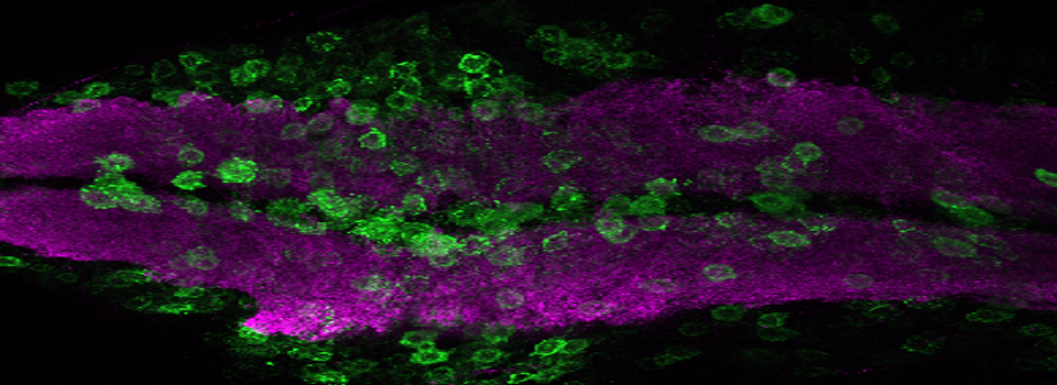
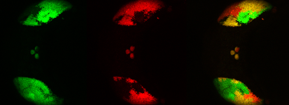
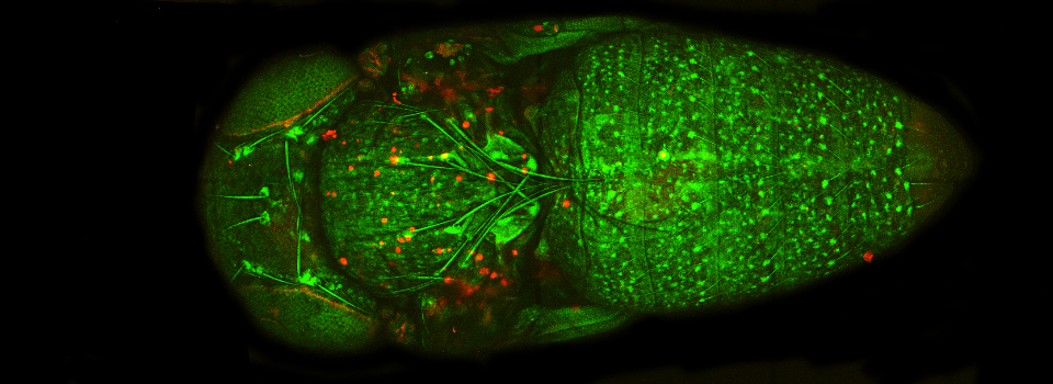
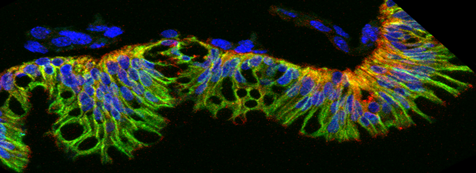
The first step is to set the lasers/detectors for the FRET donor. In this example I have used a linked CFP-YFP FRET sensor (with FRET as its default state), expressed in the mushroom body of an adult Drosophila brain. For CFP, 458nm is the best of our available laser wavelengths. Turn on the laser line (1), switch on PMT1 (2) and switch off PMT3. Use the pull down menus in PMT1 and PMT3 to call up the emission spectra for CFP and YFP, and set the detection window for PMT1 from 468nm to the left edge of the YFP curve (3). Live scan the specimen and adjust the gain/offset/laser% to get a clear image (4).

Now click “acceptor” under “Define the Acceptor setting” (1).

For YFP we use the 514nm laser. Turn the 458 to 0% and turn on the 514 (2). Activate PMT3, turn off PMT1, and set the detection window for YFP (3). Live scan again and adjust the controls until the image looks the way you want.

Now you need to set the bleach conditions. Click the “Bleach” tab on the top of the screen (1):

Turn the 514 laser to 100% (2). The “No. of frames” will determine the duration of the bleaching step (3). The optimal time will vary according to your type of specimen/ choice of FRET pairs, so you will need to experiment with various settings to find the one that works best for you. Finally, use the ROI tools (4) to select a portion of the specimen to photobleach. Click the “Run Experiment” tab at the bottom center of the panel when you are ready to begin the photobleaching protocol.

When the scan is finished the software will give you the intensities of the two fluors before and after photobleaching, as well as a calculation of FRET efficiency:

In this example, the loss of YFP and increase in CFP within the ROI are clearly visible in the images:

With the FRET Efficiency score, you can now calculate the distance (RDA) between the two fluors using this equation:

R0 is the distance required for ~50% efficiency of the maximum possible energy transfer from donor to acceptor. R0 values have been determined for many FRET pairs:

For this example the R0 for CFP-YFP is 4.7 angstroms (quite close!), and the measured efficiency was 0.4687.

This application is best used on fixed samples for calculating RDA. A live specimen (which was used in this example) will have much more variability (as the molecules will be more free to move), but it can be used to verify that a FRET sensor is functional.

2) Measuring changes in FRET ratio with the Ca Imaging Calculator

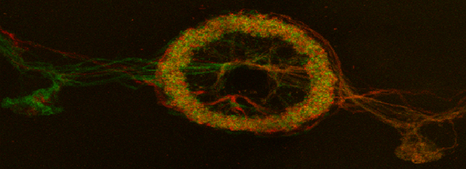
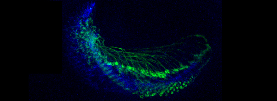
This example uses a CFP-EPac-YFP construct that changes conformation upon binding of the second messenger molecule cAMP. In the unbound state the two fluors are in close enough proximity to allow FRET between them. Upon the binding of cAMP to the EPac region, the resulting conformational shift moves the fluors further apart and reduces FRET.

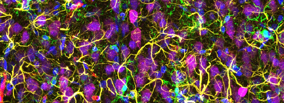
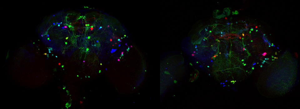
This allows for real time detection of physiological events (such as the activation of G-protein linked receptors caused by the binding of a neurotransmitter) that cause an increase in cAMP concentrations. Here the sensor was expressed in the mushroom bodies of the adult Drosophila brain via the UAS-GAL4 binary expression system (the OK107 ey driver). Dissected brain explants were placed in HL3 buffer in a well slide, and imaged with the ceramic dipping objectives. Addition of 10 μM dopamine and 10 mM acetylcholine was used to induce increases in cAMP in the responsive regions of the brains, simulating a coincident signal that comes from the combined activation of the antennal lobes (which respond to odors) and dopaminergic neurons (which respond to electric shock).

For this application the regular scanning option (TCS SP8), is used instead of one of the FRET wizards. Since the experiment will measure the change in FRET over time, the mode should be xyt or xyzt (1). With a CFP-YFP FRET pair, only the 458 laser (2), which directly excites CFP but not YFP, will be activated. However, a separate detection window for each fluor will be used. In this example, previous work has determined optimized wavelength range settings for each fluor: for CFP, PMT1 is set to 468 nm- 505 nm (3), and PMT3 is set to 524 nm- 601nm (4). For different FRET pairs you should consult the literature, but you may also wish to play with different settings to optimize them for your own experiments. The emission spectra for CFP and YFP have significant overlap (with the higher wavelength photons from CFP fluorescence mixed in with photons from the lower wavelength photons from YFP fluorescence). To compensate for this overlap, we can set up a 3rd channel that measures the ratio of YFP/ CFP fluorescence (described below).

The next step is to do a live scan; if FRET is occurring there will be images in both the CFP and YFP channels.

Set the gain, offset, zoom, Z-range, etc. The next step is to set up the Calcium Imaging calculator to create the channel that will record the ratio of YFP/CFP signal. Click the “Quantify” tab (1), select the “Stack Profile” graph option (2), and then “Calcium Imaging” from the Calculator menu (3):

Click the “analysis” tab and select the order of the channels in the ratio (1). In this example, the change in intensity of YFP (channel 2)/ CFP (channel 1) will be measured. A decrease in FRET will cause a decrease in the ratio. Next click the “Set Background” box (2):

Select the square ROI option (3), and draw a ROI in a portion of the image outside the region with EPac expression that is representative of non-specific light levels. You can activate the arrow box (4) to move the background-ROI to the best spot. You should see the numbers in the background values boxes (2) change as the ROI square is moved.

When you have selected a good background sample, unclick “set background”, then click “Calculate”. That will create a 3rd ratio channel (purple background).

The last step is to set the time parameters (and Z stack coordinates, if you are doing an xyzt scan). You should allot enough time to get a reading on the initial FRET levels before inducing any changes. The optimal length for this pre-scan, the whole scan, and the best interval between scans (i.e., how fast you are recording), will vary with each type of experiment, so consult the literature and/or try a variety of runs with different settings to determine what gets the job done. With this example, the interval is 1.293 sec, and the duration of the run is slightly more than 20 minutes, with the acetylcholine/ dopamine mixture applied to the specimen at the 2-minute mark.

The system is now ready for live imaging.

Displaying the Data

When your run is finished, you can use the “Quantify” tab (1) to view your data as a graph. Select the “Tools” tab (2) and the “Graph” tab (3).

To produce a graph of fluorescence intensity over time, you will need to draw a region of interest in the image panel. The best places for ROIs will of course vary depending on what your specimen is, and what you did to it to cause a change in FRET. In this example the 1st ROI (in green) has been drawn in a small region of the mushroom body alpha lobe, which is known to contain nerve cells that respond to inputs from PPL1 dopaminergic neurons and cholinergic projection neurons which receive signals from olfactory neurons (as mentioned above, the addition of dopamine and acetylcholine mimics that signal).

This will generate a graph for each channel and the set ratio between them:

The dopamine/acetylcholine mix was added with a pipet, which causes the downward spike in fluorescence around the 2 minute mark (likely due to the mechanical disturbance). Both channel 1 (CFP) and channel 2 (YFP), show an upward trend after this addition, but the ratio of YFP/CFP shows a strong downward trend, which indicates a loss of YFP signal relative to CFP (reduced FRET).

Multiple ROIs/ graphs can be simultaneously displayed on the same data set. Here a 2nd ROI (in purple) has been drawn on a portion of the beta lobes, where those neurons are not expected to respond to the signal as the alpha lobe neurons would.

The graph for this region (purple lines) shows that these neurons are behaving differently, as there is a small increase in the YFP/ CFP ratio:

(Thanks to Jennifer Meyers for her assistance in running this experiment.)