Co-localization in the context of fluorescence microscopy is defined as the presence of two of more fluorochromes on the same physical structure in a cell. It means that the dyes are in close proximity within a defined volume, but one must be careful in assigning any biological significance to that observation.

Some DO’s and DON’T’S in planning/performing/analysis of co-localization experiments

DO- Think carefully about the exact question you are asking. Are you trying to demonstrate that 2 proteins of interest are co-expressed in the same tissue? The same cell(s)? The same sub-cellular structures? That they are close enough to physically interact? Then be sure that you are using the right technique to answer the question. The resolving power of a confocal microscope is, on average, 200 nm laterally (x-y), and 500 nm axially (z). That means that you can analyze fluorescent signal overlap in the pixels/voxels of confocal images to make a case for co-expression on the level of tissues, cells, and larger sub-cellular compartments/organelles. Demonstration of an actual physical interaction is beyond the resolving power of this method, and techniques such as FRET should be used instead.

DO- Use the best possible objective. The higher the N/A number, the better (smaller detection volumes), and it should be corrected for chromatic aberration (the shorter the wavelength, the more the light refracts- a high quality apochromat objective will compensate for this).

DO- Use sequential scanning to minimize the effects of crosstalk (wrong excitation) and bleedthrough (wrong emission). If possible, select fluors that do not have overlapping emission spectra.

DO- Minimize noise. Use line averaging and/or slower scan speeds.

DO-Optimize your digital resolution. For the best co-localization imaging, Nyquist voxel sampling is recommended. First, find the calculated optical resolution. On the Olympus, click the Information button. On the Leica, open the Objective configuration panel. Divide these X, Y, and Z resolution values by 2.3 to get the optimal voxel size. Then adjust your voxel dimensions to match these values by adjusting the zoom ratio, scan size/format, and Z step size. The pixel (X-Y) sizes can be found in the Olympus Information panel and the X-Y panel of the Leica. The thickness of the Z-dimension will be shown in the Z-stack panels. After doing this, you can make the statement that if a single voxel contains two different colors, then those two fluorophores are within a proximity equal to or smaller than the space defined by the calculated optical resolution values.

DO- Draw regions of interest when doing quantitative analysis. Fluorescence from regions outside the cells/tissues being tested can skew the values obtained via quantitative analyses. Individual cells in a field can vary considerably in their strengths of signals due to differences in protein expression, uptake of target molecules, etc.

DO- Include positive and negative controls for comparative studies (i.e., this mutation or this drug alters protein localization). One way to generate a positive control is to co-label a protein of interest with two different fluors (100% colocalization). A simple method to generate a negative control is to rotate one of the two images 90°, then superimpose them (simulates random colocalization).

DON’T- Oversaturate your images. You should make use of the whole dynamic range, which means only the few brightest pixels should have the maximum value. Oversaturation can inflate the area/volume of a signal and give you false positives.

DON’T- use merged Z-stacks for colocalization analysis. Compression of the stacks can create false positives.

Analyzing your data- qualitative methods

Superimposing images

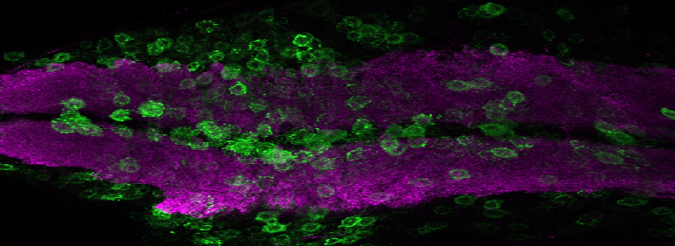
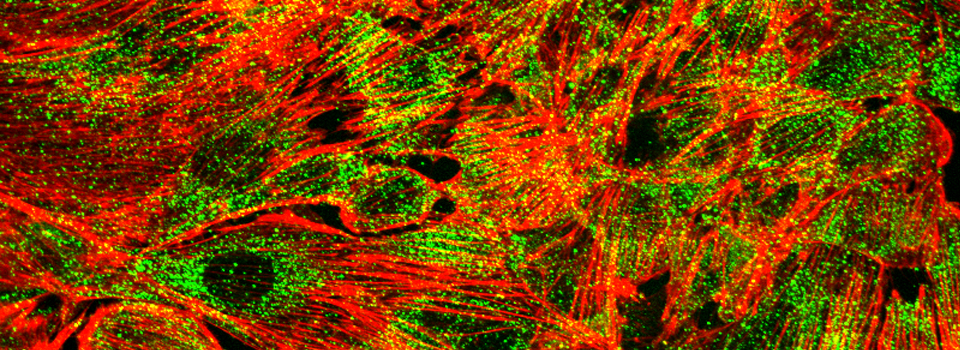
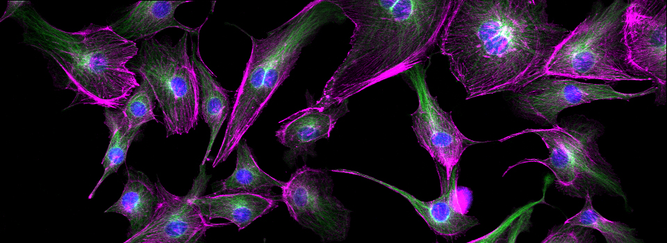
This is a common and easy way to display the data by merging channels. Regions where both fluors are present will appear as a third color, such as red and green overlaps appearing yellow or orange. Some journals prefer a green/magenta overlapping to white color scheme to accommodate readers with color blindness (assigned colors can be easily changed during processing). This is useful for visualizing the locations where the fluors overlap, and gives you a pretty picture to put in your figure. But this method by itself, in the absence of more rigorous analysis and/or using additional methods like FRET, is not enough to make a valid claim of colocalization. It is a very subjective estimate, and the results can be badly skewed by the intensities of the 2 channels.

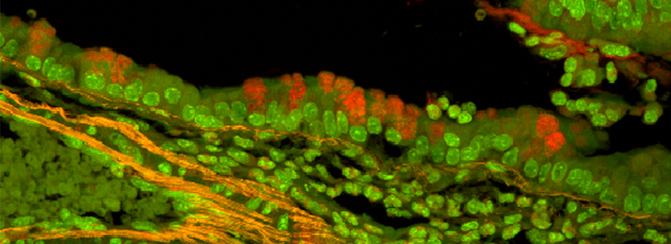
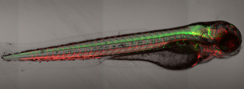
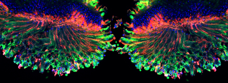
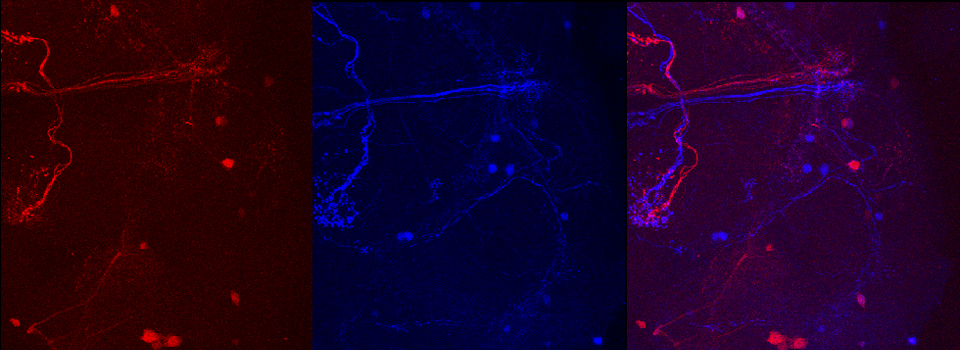
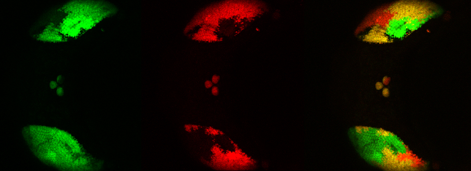
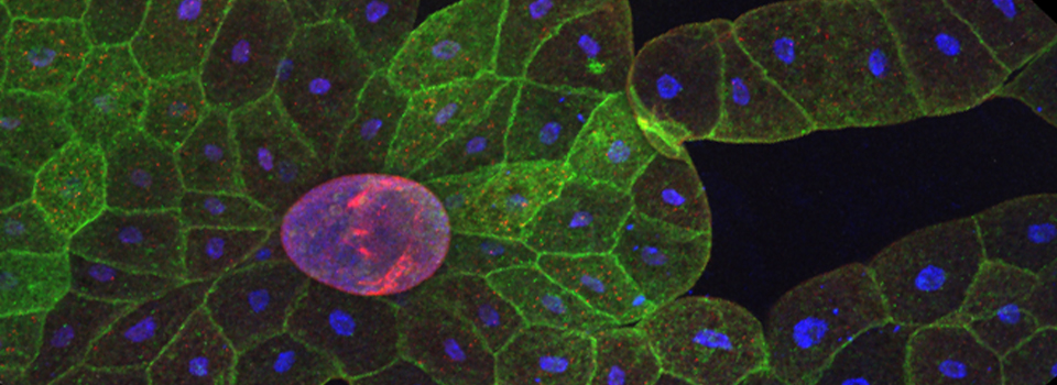
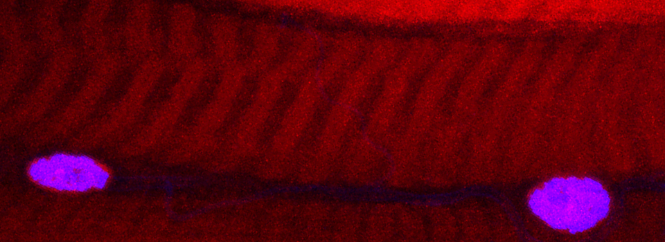
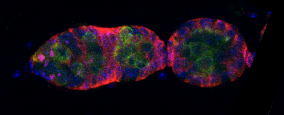
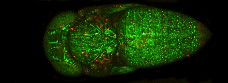
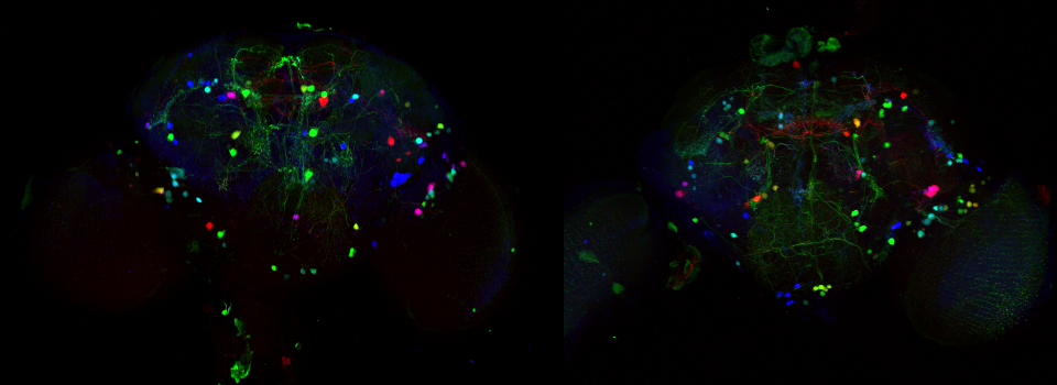
Here is an example of superimposing the images. The specimen is a Drosophila wing imaginal disc, doubled stained with red and green fluors. The image was taken on an Olympus FV1000, and the orthogonal view used to show virtual cross sections. Arrows point to patches of orange cells. You can reasonably conclude from this picture that these cells express both of the proteins detected by the fluorescent labels. But you could not conclude that these proteins physically interact or are even located in the same sub-cellular structure.

Scatter plots or Cytofluorograms

A scatterplot is two-dimensional data visualization that uses dots to represent the values obtained for two different variables - one plotted along the x-axis and the other plotted along the y-axis. In this case the variables are the intensities of the signals in the 2 fluorescent channels for each pixel. The confocal software will generate these for you when you choose co-localization mode. They can tell you the type of correlation between the two signals, and highlight any issues (noise, bleedthrough) with your images. However, this method is NOT quantitative.

Important note- these only work with 2 channels. If you imaged with 3 or more channels, you will need to de-activate the extra channels in the viewer to use the co-localization tools.

Some Cytofluorogram examples (from Leica):

(Coming up next, quantitative methods)